Computational Demonstrations: The Two-link Pendulum

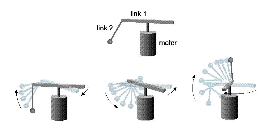
For the computer simulations, the two-segment pendulum problem (e.g., [Yamakita et al.(1995),Aamodt(1997)]) was used. The pendulum is shown in Figure 3. It has two links, a horizontal one (horizontal angle is $\alpha_1$), a coupled vertical one (vertical angle is $\alpha_2$) and a motor that is able to rotate the horizontal link in both directions. Parameters of computer illustrations are provided for the sake of reproducibility (Tables 1-3). The state of the pendulum is given by $\alpha_1$, $\alpha_2$, $\dot{\alpha}_1$ and $\dot{\alpha}_2$. For the equations of the dynamics see, e.g., the related technical report [Lorincz et al.(2002)].

The task of the learning agent was to bring up the second link into its unstable equilibrium state and balance it there. To this end, the agent could exert torque on the first link by using the motor. The agent could finish one episode by (1) reaching the goal state and stay in it for a given time interval (see Table 2) (2) reaching a time limit without success (3) violating predefined speed limits. After an episode the agent was restarted from a random state chosen from a smaller but frequently accessed domain of the state space.

The theoretically unbounded state space was limited to a finite volume by a supervising mechanism: if the agent violated a predefined angular speed limit, a penalty was applied and the agent was restarted. When the agent was in the goal state, reward zero was applied, otherwise it suffered penalty $-1$. An optimistic evaluation was used: value zero was given for every new state-state transition.

State variables were discretized by an uneven `ad hoc' partitioning of the state space. A finer discretization was used around the bottom and the top positions of the vertical link. The controller `sensed' only the code of the discretized state space. We tried different discretizations; the results shown here make use partitioning detailed in Table 3.

Figure 3: The Two-link Pendulum
Upper subfigure: the pendulum; lower subfigures: a successful episode shown in three consecutive series.

Table 1: Parameters of the Physical Model

Name of parameter	Value	Notation
Mass of horizontal link	0.82kg	$m_1$
Mass of vertical link	0.43kg	$m_2$
Length of horizontal link	0.35m	$l_1$
Length of vertical link	0.3m	$l_2$
Friction	0.005	$K^{\textit{frict}}$
Time step	0.001 ms	$\tau$
Interaction time (time between discretizations)	0.005 ms

Table 2: Reward System

Name of parameter	Value
Reward in goal state	0
Penalty in non-goal state	-1/interactions
Penalty if $\dot{\alpha}_1 > 1000$	-10 and restart
Penalty if $\dot{\alpha}_2 > 1500$	-10 and restart
Prescribed Standing Time	10 s
Goal state if	$\alpha_2<\pm ~ 12^\circ$
	$\dot{\alpha}_2 < \pm ~ 60^\circ/$sec

Table 3: Learning Parameters

Name of parameter	Value	Notation
Learning rate	0.02	$\alpha$
Discount factor	0.95	$\gamma$
SDS feedback gain	0.0-10.0	$\Lambda$
SDS weighting factor	0.9	$\alpha_{SDS}$
Eligibility decay	0.8	$\lambda$
Eligibility depth	70 steps
Number of partitions in $\alpha_1$, $\alpha_2$, $\dot{\alpha}_1$ and $\dot{\alpha}_2$	1, 16, 6, 14
Base control actions	$\pm$ 1.5 Nm
Average frequency of random control action	2 Hz
Maximal episode length	60 sec

In the experiments, the E-learning algorithm with the SDS controller was used. The inverse dynamics had two base actions, which were corrected by the SDS controller. First the agent learned the inverse dynamics by experience: a random base action was selected then the system was periodically restarted in 10 second intervals from random positions. In every time step, the 4-dimensional state vector of the underlying continuous state space was transformed into a 4-dimensional discrete state vector according to the predefined partitioning of the state space dimensions. In this reduced state space, a transition (event) happens if the system's trajectory crosses any boundary of the predefined partitioning. When no boundaries were crossed, the agent experienced an $(x_t, x_t)$ transition or event (the agent remained in the same state). The system recorded how many times an event happened for the different base actions. The inverse dynamics for an event are given by the most likely action when the event occurs. After some time, the number of the newly experienced transitions was not increased significantly. Then we stopped the tuning of the inverse dynamics and started learning in the RL framework (see Table 3 for the learning parameters). To accelerate learning, eligibility traces were used. The agent could select only the experienced events from a given position. Computations simulated real time.