Next: Decomposable priors and MAP
Up: Mixtures of trees
Previous: Running time
Learning mixtures of trees with shared structure
It is possible to modify the MIXTREE algorithm so as to
constrain the  trees to share the same structure, and thereby
estimate MTSS models.
The E step remains unchanged. The only novelty is the reestimation of
the tree distributions
trees to share the same structure, and thereby
estimate MTSS models.
The E step remains unchanged. The only novelty is the reestimation of
the tree distributions  in the M step, since they are now
constrained to have the same structure. Thus, the maximization cannot
be decoupled into separate tree estimations but, remarkably
enough, it can still be performed efficiently.
It can be readily verified that for any given structure the optimal
parameters of each tree edge
in the M step, since they are now
constrained to have the same structure. Thus, the maximization cannot
be decoupled into separate tree estimations but, remarkably
enough, it can still be performed efficiently.
It can be readily verified that for any given structure the optimal
parameters of each tree edge  are equal to the parameters of
the corresponding marginal distribution
are equal to the parameters of
the corresponding marginal distribution  . It remains only
to find the optimal structure. The expression to be optimized is the
second sum in the right-hand side of equation (7). By
replacing with and denoting the mutual
information between
. It remains only
to find the optimal structure. The expression to be optimized is the
second sum in the right-hand side of equation (7). By
replacing with and denoting the mutual
information between  and
and  under
under  by
by  this sum can
be reexpressed as follows:
this sum can
be reexpressed as follows:
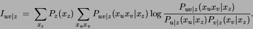
The new quantity  appearing above represents the mutual
information of and conditioned on the hidden variable
appearing above represents the mutual
information of and conditioned on the hidden variable  . Its
general definition for three discrete variables
. Its
general definition for three discrete variables  distributed
according to
distributed
according to
 is
is
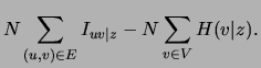
The second term in (8),
 ,
represents the sum of the conditional entropies of the variables given
and is independent of the tree structure. Hence, the optimization
of the structure
,
represents the sum of the conditional entropies of the variables given
and is independent of the tree structure. Hence, the optimization
of the structure  can be achieved by running a MWST algorithm with the
edge weights represented by . We summarize the algorithm in
Figure 7.
can be achieved by running a MWST algorithm with the
edge weights represented by . We summarize the algorithm in
Figure 7.
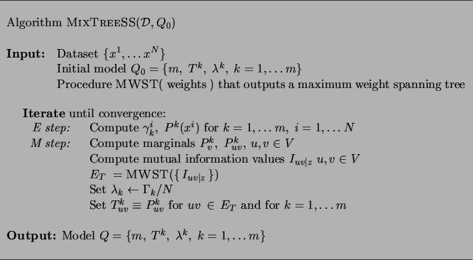
Figure 7:
The MIXTREESS algorithm for learning MTSS models.
 |
Next: Decomposable priors and MAP
Up: Mixtures of trees
Previous: Running time
Journal of Machine Learning Research
2000-10-19
![$\displaystyle N\sum_{k=1}^m \lambda_k [\sum_{(u,v)\in E}I^k_{uv} -
\sum_{v \in V} H(P^k_v)]$](img164.png)