Learning of MT models

The expectation-maximization (EM) algorithm provides an effective approach to solving many learning problems [Dempster, Laird, Rubin 1977,MacLachlan, Bashford 1988], and has been employed with particular success in the setting of mixture models and more general latent variable models [Jordan, Jacobs 1994,Jelinek 1997,Rubin, Thayer 1983]. In this section we show that EM also provides a natural approach to the learning problem for the MT model. An important feature of the solution that we present is that it provides estimates for both parametric and structural aspects of the model. In particular, although we assume (in the current section) that the number of trees is fixed, the algorithm that we derive provides estimates for both the pattern of edges of the individual trees and their parameters. These estimates are maximum likelihood estimates, and although they are subject to concerns about overfitting, the constrained nature of tree distributions helps to ameliorate overfitting problems. It is also possible to control the number of edges indirectly via priors; we discuss methods for doing this in Section 4. We are given a set of observations ${\cal D}=\{x^1, x^2, \ldots, x^N\}$ and are required to find the mixture of trees $Q$ that satisfies

$$Q\;=\;\mbox{\raisebox{-1.7ex}{$\stackrel{\textstyle {\rm argmax}}{\scriptstyle Q'}$}} \sum_{i=1}^N \log Q(x^i).$$

Within the framework of the EM algorithm, this likelihood function is referred to as the incomplete log-likelihood and it is contrasted with the following complete log-likelihood function:

$$l_c( x^{1,\ldots N}, z^{1,\ldots N}\vert Q) = \sum_{i=1}^N \log \prod_{k=1}^m (\lambda _k T^k (x^i))^{\delta_{k,z^i}}$$

$$= \sum_{i=1}^N \sum_{k=1}^m \delta_{k,z^i} (\log \lambda _k + \log T^k (x^i)),$$ (5)

where $\delta_{k,z^i}$ is equal to one if $z^i$ is equal to the $k$th value of the choice variable and zero otherwise. The complete log-likelihood would be the log-likelihood of the data if the unobserved data $\{z^1, z^2, \ldots, z^N\}$ could be observed. The idea of the EM algorithm is to utilize the complete log-likelihood, which is generally easy to maximize, as a surrogate for the incomplete log-likelihood, which is generally somewhat less easy to maximize directly. In particular, the algorithm goes uphill in the expected value of the complete log-likelihood, where the expectation is taken with respect to the unobserved data. The algorithm thus has the form of an interacting pair of steps: the E step, in which the expectation is computed given the current value of the parameters, and the M step, in which the parameters are adjusted so as to maximize the expected complete log-likelihood. These two steps iterate and are proved to converge to a local maximum of the (incomplete) log-likelihood [Dempster, Laird, Rubin 1977]. Taking the expectation of (5), we see that the E step for the MT model reduces to taking the expectation of the delta function $\delta_{k,z^i}$, conditioned on the data ${\cal D}$:

$$E[ \delta_{k,z^i} \vert {\cal D} ] = Pr[ z^i = k \vert {\cal D} ] = Pr[ z^i = k \vert V = x^i ],$$

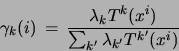
and this latter quantity is recognizable as the posterior probability of the hidden variable given the $i$th observation (cf. equation (4)). Let us define:

$$\gamma_k(i) = \frac{\lambda_k T^k(x^i)}{\sum_{k'}\lambda_{k'}T^{k'}(x^i)}$$ (6)

as this posterior probability. Substituting (6) into the expected value of the complete log-likelihood in (5), we obtain:

$$E[l_c( x^{1,\ldots N}, z^{1,\ldots N}\vert Q)]\;=\; \sum_{i... ...um_{k=1}^m \gamma_k(i) (\log \lambda _k + \log T^k (x^i)).$$

Let us define the following quantities:

$$\Gamma_k = \sum_{i=1}^N \gamma_k(x^i),\;\;\;k=1,\ldots m$$

$$P^k(x^i) = \frac{\gamma_k(i)}{\Gamma_k},$$

where the sums $\Gamma_k \in [0,N]$ can be interpreted as the total number of data points that are generated by component $T^k$. Using these definitions we obtain:

$$E[l_c(x^{1,\ldots N}, z^{1,\ldots N} \vert Q)] \;=\; \su... ...\sum_{k=1}^m \Gamma_k \sum_{i=1}^N P^k(x^i)\log T^k(x^i).$$ (7)

It is this quantity that we must maximize with respect to the parameters.

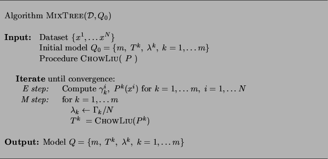
Figure 6: The MIXTREE algorithm for learning MT models.

From (7) we see that $E[l_c]$ separates into terms that depend on disjoint subsets of the model parameters and thus the M step decouples into separate maximizations for each of the various parameters. Maximizing the first term of (7) with respect to the parameters $\lambda$, subject to the constraint $\sum_{k=1}^m \lambda_k\;=\; 1$, we obtain the following update equation:

$$\lambda_k\;=\;\frac{\Gamma_k}{N} \;\;{\rm for }\;k=1,\ldots m.$$

In order to update $T^k$, we see that we must maximize the negative cross-entropy between $P^k$ and $T^k$:

$$\sum_{i=1}^N P^k(x^i)\log T^k(x^i).$$

This problem is solved by the CHOWLIU algorithm from Section 2.3. Thus we see that the M step for learning the mixture components of MT models reduces to $m$ separate runs of the CHOWLIU algorithm, where the ``target'' distribution $P^k(x^i)$ is the normalized posterior probability obtained from the E step. We summarize the results of the derivation of the EM algorithm for mixtures of trees in Figure 6.