Next: Mixtures of trees
Up: Tree distributions
Previous: Representational capabilities
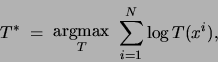
Learning of tree distributions
The learning problem is formulated as follows: we are given a set of
observations
 and we are
required to find the tree
and we are
required to find the tree  that maximizes the log likelihood of
the data:
that maximizes the log likelihood of
the data:
where  is an assignment of values to all variables.
Note that the maximum is taken both with respect to the
tree structure (the choice of which edges to include) and with respect
to the numerical values of the parameters. Here and in the rest of
the paper we will assume for simplicity that there are no missing values
for the variables in
is an assignment of values to all variables.
Note that the maximum is taken both with respect to the
tree structure (the choice of which edges to include) and with respect
to the numerical values of the parameters. Here and in the rest of
the paper we will assume for simplicity that there are no missing values
for the variables in  , or, in other words, that the observations
are complete.
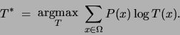
Letting
, or, in other words, that the observations
are complete.
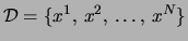
Letting  denote the proportion of observations
  in the
training set
in the
training set  that are equal to
  , we can alternatively
express the maximum likelihood problem by summing over configurations
:
, we can alternatively
express the maximum likelihood problem by summing over configurations
:
In this form we see that the log likelihood criterion function is
a (negative) cross-entropy. We will in fact solve the problem in
general, letting be an arbitrary probability distribution.
This generality will prove useful in the following section where
we consider mixtures of trees.
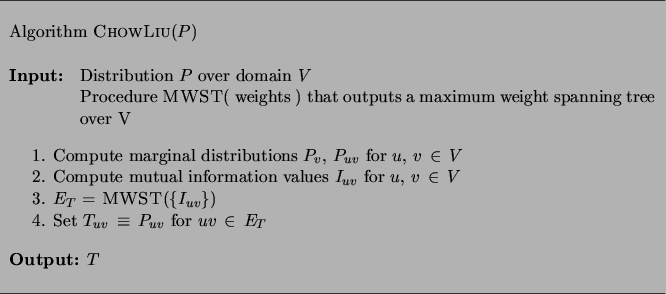
The solution to the learning problem is an algorithm, due to[Chow, Liu 1968] ,
that has quadratic complexity in  (see Figure 3).
There are three steps to the algorithm.
First, we compute the pairwise marginals
(see Figure 3).
There are three steps to the algorithm.
First, we compute the pairwise marginals
 .
If
.
If  is an empirical distribution, as in the present case, computing
these marginals requires
is an empirical distribution, as in the present case, computing
these marginals requires
 operations.
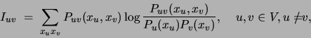
Second, from these marginals we compute the mutual information
between each pair of variables in under the distribution :
operations.
Second, from these marginals we compute the mutual information
between each pair of variables in under the distribution :
an operation that requires
 operations. Third,
we run a maximum-weight spanning tree (MWST) algorithm [Cormen, Leiserson, Rivest
1990],
using
operations. Third,
we run a maximum-weight spanning tree (MWST) algorithm [Cormen, Leiserson, Rivest
1990],
using  as the weight for edge
 .
Such algorithms, which run in time
.
Such algorithms, which run in time  , return a spanning tree
that maximizes the total mutual information for edges included in
the tree.
, return a spanning tree
that maximizes the total mutual information for edges included in
the tree.
Figure 3:
The Chow and Liu algorithm for maximum likelihood
estimation of tree structure and parameters.
 |
Chow and Liu showed that the maximum-weight spanning tree
also maximizes the likelihood over tree distributions  , and
moreover the optimizing parameters
, and
moreover the optimizing parameters  (or
(or  ),
for
),
for
 , are equal to the corresponding marginals
 of the distribution :
The algorithm thus attains a global optimum over both structure
and parameters.
Next: Mixtures of trees
Up: Tree distributions
Previous: Representational capabilities
Journal of Machine Learning Research
2000-10-19