Next: Experiments
Up: Decomposable priors and MAP
Previous: Decomposable priors for tree
The decomposable prior for parameters that we introduce is a
Dirichlet prior [Heckerman, Geiger, Chickering
1995]. The Dirichlet distribution
is defined over the domain of
 and has the form
The numbers
 that parametrize
  can be interpreted as the sufficient statistics of a ``fictitious
data set'' of size
can be interpreted as the sufficient statistics of a ``fictitious
data set'' of size
 . Therefore
  are called
fictitious counts.
are called
fictitious counts.  represents the strength of the prior.
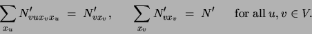
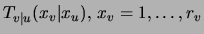
To specify a prior for tree parameters, one must
specify a Dirichlet distribution for each of the
probability tables
represents the strength of the prior.
To specify a prior for tree parameters, one must
specify a Dirichlet distribution for each of the
probability tables
 , for each possible tree structure
  . This is achieved by
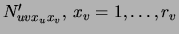
means of a set of parameters
. This is achieved by
means of a set of parameters  satisfying
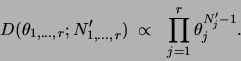
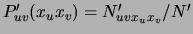
With these settings, the prior for the parameters
 in any tree that contains the directed edge
 is defined by
 . This
representation of the prior is not only compact (order
. This
representation of the prior is not only compact (order  parameters) but it is
also consistent: two different directed parametrizations of the same
tree distribution receive the same prior. The assumptions allowing us to
define this prior are explicated by MJa:uai00 and
parallel the reasoning of heckerman:95 for general Bayes nets.
Denote by
parameters) but it is
also consistent: two different directed parametrizations of the same
tree distribution receive the same prior. The assumptions allowing us to
define this prior are explicated by MJa:uai00 and
parallel the reasoning of heckerman:95 for general Bayes nets.
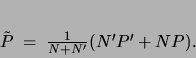
Denote by  the empirical distribution obtained from a data set of
size
the empirical distribution obtained from a data set of
size  and by
 the
distribution defined by the fictitious counts. Then, by a property of the Dirichlet distribution [Heckerman, Geiger, Chickering
1995] it follows that learning a MAP tree
is equivalent to learning an ML tree for the weighted
combination
the
distribution defined by the fictitious counts. Then, by a property of the Dirichlet distribution [Heckerman, Geiger, Chickering
1995] it follows that learning a MAP tree
is equivalent to learning an ML tree for the weighted
combination  of the two ``datasets''
 |
(10) |
Consequently, the parameters of the optimal tree will be
 .
For a mixture of trees, maximizing the posterior translates into
replacing by
.
For a mixture of trees, maximizing the posterior translates into
replacing by  and by
  in equation
(10) above. This implies that the M
step of the EM algorithm, as well as the E step, is exact and
tractable in the case of MAP estimation with decomposable
priors.
Finally, note that the posteriors
in equation
(10) above. This implies that the M
step of the EM algorithm, as well as the E step, is exact and
tractable in the case of MAP estimation with decomposable
priors.
Finally, note that the posteriors
![$Pr[ Q\vert{\cal D}]$](img172.png) for models
with different
for models
with different  are defined up to a constant that depends on
. Hence, one cannot compare posteriors of MTs with different
numbers of mixture components . In the experiments that
we present, we chose via other performance criteria:
validation set likelihood in the density estimation experiments
and validation set classification accuracy in the classification
tasks.
are defined up to a constant that depends on
. Hence, one cannot compare posteriors of MTs with different
numbers of mixture components . In the experiments that
we present, we chose via other performance criteria:
validation set likelihood in the density estimation experiments
and validation set classification accuracy in the classification
tasks.
Next: Experiments
Up: Decomposable priors and MAP
Previous: Decomposable priors for tree
Journal of Machine Learning Research
2000-10-19