Decomposable priors for tree structures

The general form of a decomposable prior for the tree structure $E$ is one where each edge contributes a constant factor independent of the presence or absence of other edges in $E$:

$$Pr[E] \;\propto\; \prod_{{(u,v) \in E}} \exp(-\beta_{uv}).$$

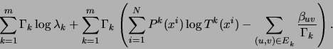
With this prior, the expression to be maximized in the M step of the EM algorithm becomes

$$\sum_{k=1}^m \Gamma_k \log \lambda_k +\sum_{k=1}^m \Gamma_k... ... \sum_{{(u,v) \in E}_k} \frac{\beta_{uv}}{\Gamma_k}\right).$$

Consequently, each edge weight $W_{uv}^k$ in tree $T_k$ is adjusted by the corresponding value $\beta_{uv}$ divided by the total number of points that tree $k$ is responsible for:

$$W_{uv}^k \;=\;I_{uv}^k \;-\; \frac{\beta_{uv}}{\Gamma_k}.$$

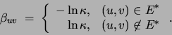
A negative $\beta_{uv}$ increases the probability of $(u,v)$ being present in the final solution, whereas a positive value of $\beta_{uv}$ acts like a penalty on the presence of edge $(u,v)$ in the tree. If the MWST procedure is modified so as to not add negative-weight edges, one can obtain (disconnected) trees having fewer than $n-1$ edges. Note that the strength of the prior is inversely proportional to $\Gamma_k$, the total number of data points assigned to mixture component $k$. Thus, with equal priors for all trees $T^k$, trees accounting for fewer data points will be penalized more strongly and therefore will be likely to have fewer edges. If one chooses the edge penalties to be proportional to the increase in the number of parameters caused by the addition of edge $uv$ to the tree,

$$\beta_{uv}\;=\;\frac{1}{2}(r_u-1)(r_v-1)\log N$$

then a Minimum Description Length (MDL) [Rissanen 1989] type of prior is implemented. In the context of learning Bayesian networks, heckerman:95 suggested the following prior:

$$Pr[ E] \; \propto \; \kappa^{\Delta(E,E^{\ast})}$$

where $\Delta(\cdot)$ is a distance metric between Bayes net structures and $E^\ast$ is the prior network structure. Thus, this prior penalizes deviations from the prior network. This prior is decomposable, entailing

$$\beta_{uv}\;=\;\left\{\begin{array}{rl}-\ln \kappa, & {(u,v... ...\ast\\ \ln \kappa, & (u,v)\not\in E^\ast\end{array}\right..$$

Decomposable priors on structure can also be used when the structure is common for all trees (MTSS). In this case the effect of the prior is to penalize the weight $I_{uv\vert z}$ in (8) by $-\beta_{uv}/{N}$. A decomposable prior has the remarkable property that its normalization constant can be computed exactly in closed form. This makes it possible not only to completely define the prior, but also to compute averages under this prior (e.g., to compute a model's evidence). Given that the number of all undirected tree structures over $n$ variables is $n^{n-2}$, this result [Meila, Jaakkola 2000] is quite surprising.