The implementation of LSVM is straightforward, as shown in the
previous sections. Our first ``dry run" experiments were on randomly
generated problems just to test the speed and effectiveness of LSVM on
large problems. We first used a Pentium III 500 MHz notebook with 384
megabytes of memory (and additional swap space) on 2
million randomly generated points in ![]() with
with
![]() and
and
![]() . LSVM solved the problem in 6 iterations
in 81.52 minutes to an optimality criterion of
. LSVM solved the problem in 6 iterations
in 81.52 minutes to an optimality criterion of ![]() on a 2-norm
violation of (14). The same problem was solved in the same
number of iterations and to the same accuracy in
on a 2-norm
violation of (14). The same problem was solved in the same
number of iterations and to the same accuracy in ![]() minutes on a
250 MHz UltraSPARC II processor with 2 gigabytes of memory. After
these preliminary encouraging tests we proceeded to more systematic
numerical tests as follows.
minutes on a
250 MHz UltraSPARC II processor with 2 gigabytes of memory. After
these preliminary encouraging tests we proceeded to more systematic
numerical tests as follows.
Most of the rest of our experiments were run on the Carleton College workstation ``gray'', which utilizes a 700 MHz Pentium III Xeon processor and a maximum of 2 Gigabytes of memory available for each process. This computer runs Redhat Linux 6.2, with MATLAB 6.0. The one set of experiments showing the checkerboard were run on the UW-Madison Data Mining Institute ``locop2'' machine, which utilizes a 400 MHz Pentium II Xeon and a maximum of 2 Gigabytes of memory available for each process. This computer runs Windows NT Server 4.0, with MATLAB 5.3.1. Both gray and locop2 are multiprocessor machines. However, only one processor was used for all the experiments shown here as MATLAB is a single threaded application and does not distribute any effort across processors [27]. We had exclusive access to these machines, so there were no issues with other users inconsistently slowing the computers down.
The first results we present are designed to show that our
reformulation of the SVM (7) and its associated algorithm
LSVM yield similar performance to the standard SVM (2),
referred to here as SVM-QP. Results are also shown for our active set
SVM (ASVM) algorithm [18]. For six
datasets available from the UCI Machine Learning Repository
[22], we performed tenfold cross validation in order to
compare test set accuracies between the methodologies. Furthermore, we
utilized a tuning set for each algorithm to find the optimal value of
the parameter ![]() . For both LSVM and ASVM, we used an optimality
tolerance of 0.001 to determine when to terminate. SVM-QP was
implemented using the high-performing CPLEX barrier quadratic
programming solver [9] with its default stopping
criterion. Altering the CPLEX default stopping criterion to match that
of LSVM did not result in significant change in timing relative to
LSVM, but did reduce test set correctness for SVM-QP.
. For both LSVM and ASVM, we used an optimality
tolerance of 0.001 to determine when to terminate. SVM-QP was
implemented using the high-performing CPLEX barrier quadratic
programming solver [9] with its default stopping
criterion. Altering the CPLEX default stopping criterion to match that
of LSVM did not result in significant change in timing relative to
LSVM, but did reduce test set correctness for SVM-QP.
We also tested SVM-QP with the well-known optimized algorithm
SVM![]() [10]. Joachims, the author of SVM
[10]. Joachims, the author of SVM![]() ,
graciously provided us with the newest version of the software
(Version 3.10b) and advice on setting the parameters. All features for
all experiments were normalized to the range
,
graciously provided us with the newest version of the software
(Version 3.10b) and advice on setting the parameters. All features for
all experiments were normalized to the range ![]() as recommended
in the SVM
as recommended
in the SVM![]() documentation. Such normalization was used in all
experiments that we present, and is recommended for the LSVM algorithm
due to the penalty on the bias parameter
documentation. Such normalization was used in all
experiments that we present, and is recommended for the LSVM algorithm
due to the penalty on the bias parameter ![]() which we have added
to our objective (7). We chose to use the default
termination error criterion in SVM
which we have added
to our objective (7). We chose to use the default
termination error criterion in SVM![]() of
of ![]() . We also
present an estimate of how much memory each algorithm used, as well as
the number of support vectors. The number of support vectors was
determined here as the number of components of the dual vector
. We also
present an estimate of how much memory each algorithm used, as well as
the number of support vectors. The number of support vectors was
determined here as the number of components of the dual vector ![]() that were nonzero. Moreover, we also present the number of components
of
that were nonzero. Moreover, we also present the number of components
of ![]() larger than 0.001 (referred to in the table as ``SVs with
tolerance'').
larger than 0.001 (referred to in the table as ``SVs with
tolerance'').
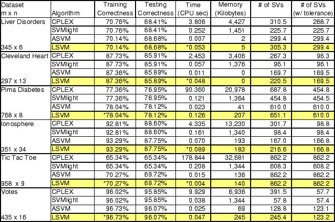
The results demonstrate that LSVM performs comparably to SVM-QP with
respect to generalizability, and shows running times comparable to or
better than SVM![]() . LSVM and ASVM show nearly identical
generalization performance, as they solve the same optimization
problem. Any differences in generalization observed between the two
are only due to different approximate solutions being found at
termination. LSVM and ASVM usually run in roughly the same amount of
time, though there are some cases where ASVM is noticeably faster than
LSVM. Nevertheless, this is impressive performance on the part of
LSVM, which is a dramatically simpler algorithm than ASVM, CPLEX, and
SVM
. LSVM and ASVM show nearly identical
generalization performance, as they solve the same optimization
problem. Any differences in generalization observed between the two
are only due to different approximate solutions being found at
termination. LSVM and ASVM usually run in roughly the same amount of
time, though there are some cases where ASVM is noticeably faster than
LSVM. Nevertheless, this is impressive performance on the part of
LSVM, which is a dramatically simpler algorithm than ASVM, CPLEX, and
SVM![]() . LSVM utilizes significantly less memory than the SVM-QP
algorithms as well, though it does require more support
vectors than SVM-QP. We address this point in the conclusion.
. LSVM utilizes significantly less memory than the SVM-QP
algorithms as well, though it does require more support
vectors than SVM-QP. We address this point in the conclusion.
 |
 |
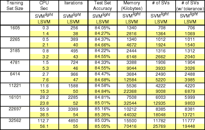
We next compare LSVM with SVM![]() on the Adult dataset
[22], which is commonly used to compare SVM algorithms
[24,17]. These results, shown in Table 2,
demonstrate that for the largest training sets LSVM performs faster
than SVM
on the Adult dataset
[22], which is commonly used to compare SVM algorithms
[24,17]. These results, shown in Table 2,
demonstrate that for the largest training sets LSVM performs faster
than SVM![]() with similar test set accuracies. Note that the
``iterations'' column takes on very different meanings for the two
algorithms. SVM
with similar test set accuracies. Note that the
``iterations'' column takes on very different meanings for the two
algorithms. SVM![]() defines an iteration as solving an
optimization problem over a a small number, or ``chunk,'' of
constraints. LSVM, on the other hand, defines an iteration as a matrix
calculation which updates all the dual variables simultaneously. These
two numbers are not directly comparable, and are included here only
for purposes of monitoring scalability. In this experiment, LSVM
uses significantly more memory than SVM
defines an iteration as solving an
optimization problem over a a small number, or ``chunk,'' of
constraints. LSVM, on the other hand, defines an iteration as a matrix
calculation which updates all the dual variables simultaneously. These
two numbers are not directly comparable, and are included here only
for purposes of monitoring scalability. In this experiment, LSVM
uses significantly more memory than SVM![]() .
.
Table 3 shows results from running LSVM on a massively sized
dataset. This dataset was created using our own NDC Data Generator
[23] as suggested by Usama Fayyad. The results show that LSVM
can be used to solve massive problems quickly, which is particularly
intriguing given the simplicity of the LSVM Algorithm. Note that for
these experiments, all the data was brought into memory. As such, the
running time reported consists of the time used to actually solve the
problem to termination excluding I/O time. This is consistent with
the measurement techniques used by other popular approaches
[11,24]. Putting all the data in memory is simpler to code
and results in faster running times. However, it is not a fundamental
requirement of our algorithm -- block matrix multiplications,
incremental evaluations of ![]() using another application of the
Sherman-Morrison-Woodbury identity, and indices on the dataset can be
used to create an efficient disk based version of LSVM. We note
that we tried to run SVM
using another application of the
Sherman-Morrison-Woodbury identity, and indices on the dataset can be
used to create an efficient disk based version of LSVM. We note
that we tried to run SVM![]() on this dataset, but after running
for more than six hours it did not terminate.
on this dataset, but after running
for more than six hours it did not terminate.
We now demonstrate the effectiveness of LSVM in solving nonlinear
classification problems through the use of kernel functions. One highly
nonlinearly separable but simple example is the ``tried and true''
checkerboard dataset [8], which has often been used to show
the effectiveness of nonlinear kernel methods on a dataset for which a
linear separation clearly fails. The checkerboard dataset contains
1000 points randomly sampled from a checkerboard. These points are
used as a training set in LSVM to try to reproduce an accurate
rendering of a checkerboard. For this problem, we used the following
Gaussian kernel:
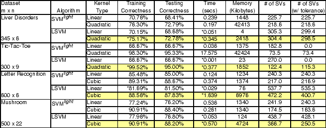
The final set of experiments, shown in Table 4, demonstrates the effectiveness of nonlinear kernel functions with LSVM on UCI datasets [22] specialized as follows for purposes of our tests:
We chose which kernels to use and appropriate values of ![]() via
tuning sets and tenfold cross-validation techniques. The results show
that nonlinear kernels produce test set accuracies that improve on
those obtained with linear kernels.
via
tuning sets and tenfold cross-validation techniques. The results show
that nonlinear kernels produce test set accuracies that improve on
those obtained with linear kernels.
 |