


Next: Density estimation experiments
Up: Structure identification
Previous: Random trees, large data
The ``bars'' problem is a benchmark structure learning problem
for unsupervised learning algorithms in the neural network
literature [Dayan, Zemel 1995].
Figure 8:
Eight training examples for the bars learning task.
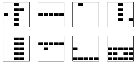 |
The domain  is the
  square of binary variables depicted
in Figure 8. The data are generated in the following
manner: first, one flips a fair coin to decide whether to generate
horizontal or vertical bars; this represents the hidden variable in
our model. Then, each of the
square of binary variables depicted
in Figure 8. The data are generated in the following
manner: first, one flips a fair coin to decide whether to generate
horizontal or vertical bars; this represents the hidden variable in
our model. Then, each of the  bars is turned on independently
(black in Figure 8) with probability
bars is turned on independently
(black in Figure 8) with probability  .
Finally, noise is added by flipping each bit of the image independently
with probability
.
Finally, noise is added by flipping each bit of the image independently
with probability  . A learner is shown data generated by this
process; the task of the learner is to discover the data generating mechanism.
. A learner is shown data generated by this
process; the task of the learner is to discover the data generating mechanism.
Figure 9:
The true structure of the probabilistic generative model for the bars data.
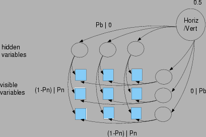 |
Figure 10:
A mixture of trees that approximates the generative model for the bars
problem. The interconnection between the variables in each ``bar'' are
arbitrary.
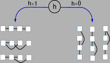 |
A mixture of trees model that approximates the true structure for low
noise levels is shown in Figure 10. Note that any
tree over the variables forming a bar is an equally good approximation.
Thus, we will consider that the structure has been discovered when the model
learns a mixture with  , each
  having connected components,
one for each bar. Additionally, we shall test the classification
accuracy of the learned model by comparing the true value of the
hidden variable (i.e. ``horizontal'' or ``vertical'') with the value
estimated by the model for each data point in a test set.
As seen in the first row, third column of Figure 8, some
training set examples are ambiguous. We retained these ambiguous
examples in the training set. The total training set size was
having connected components,
one for each bar. Additionally, we shall test the classification
accuracy of the learned model by comparing the true value of the
hidden variable (i.e. ``horizontal'' or ``vertical'') with the value
estimated by the model for each data point in a test set.
As seen in the first row, third column of Figure 8, some
training set examples are ambiguous. We retained these ambiguous
examples in the training set. The total training set size was
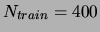 . We trained models with
 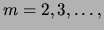 and evaluated
the models on a validation set of size 100 to choose the final values
of
and evaluated
the models on a validation set of size 100 to choose the final values
of  and of the smoothing parameter
  . Typical values for
in the literature are
. Typical values for
in the literature are  ; we choose
  following
dayan:95. The other parameter values were
following
dayan:95. The other parameter values were
 and
and  . To obtain trees with several connected components
we used a small edge penalty
. To obtain trees with several connected components
we used a small edge penalty  .
.
Figure 11:
Test set log-likelihood on the bars learning task for different values
of the smoothing parameter and different . The figure
presents averages and standard deviations over 20 trials.
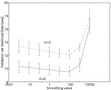 |
The validation-set log-likelihoods (in bits) for
 are given in Figure 11. Clearly, is
the best model.
For we examined the resulting
structures: in 19 out of 20 trials, structure recovery was perfect.
Interestingly, this result held for the whole range of the smoothing
parameter , not simply at the cross-validated value. By way of
comparison, dayan:95 examined two training methods and the
structure was recovered in 27 and respectively 69 cases out of 100.
The ability of the learned representation to categorize new examples
as coming from one group or the other is referred to as classification
performance and is shown in Table 1. The result
reported is obtained on a separate test set for the final,
cross-validated value of . Note that, due to the presence of
ambiguous examples, no model can achieve perfect classification. The
probability of an ambiguous example is
are given in Figure 11. Clearly, is
the best model.
For we examined the resulting
structures: in 19 out of 20 trials, structure recovery was perfect.
Interestingly, this result held for the whole range of the smoothing
parameter , not simply at the cross-validated value. By way of
comparison, dayan:95 examined two training methods and the
structure was recovered in 27 and respectively 69 cases out of 100.
The ability of the learned representation to categorize new examples
as coming from one group or the other is referred to as classification
performance and is shown in Table 1. The result
reported is obtained on a separate test set for the final,
cross-validated value of . Note that, due to the presence of
ambiguous examples, no model can achieve perfect classification. The
probability of an ambiguous example is
 , which yields an error rate
of
, which yields an error rate
of
 . Comparing this lower bound with the value in
the corresponding column of Table 1 shows that
the model performs quite well, even when trained on ambiguous
examples.
To further support this conclusion, a second test set of size 200 was
generated, this time including only non-ambiguous examples. The
classification performance, shown in the corresponding section of
Table 1, rose to 0.95. The table also shows the
likelihood of the (test) data evaluated on the learned model. For the
first, ``ambiguous'' test set, this is 9.82, 1.67 bits away from the true
model likelihood of 8.15 bits/data point. For the ``non-ambiguous'' test
set, the compression rate is significantly worse, which is not surprising
given that the distribution of the test set is now different from the
distribution the model was trained on.
. Comparing this lower bound with the value in
the corresponding column of Table 1 shows that
the model performs quite well, even when trained on ambiguous
examples.
To further support this conclusion, a second test set of size 200 was
generated, this time including only non-ambiguous examples. The
classification performance, shown in the corresponding section of
Table 1, rose to 0.95. The table also shows the
likelihood of the (test) data evaluated on the learned model. For the
first, ``ambiguous'' test set, this is 9.82, 1.67 bits away from the true
model likelihood of 8.15 bits/data point. For the ``non-ambiguous'' test
set, the compression rate is significantly worse, which is not surprising
given that the distribution of the test set is now different from the
distribution the model was trained on.
Table 1:
Results on the bars learning task.
| Test set |
ambiguous |
unambiguous |
 [bits/datapt] [bits/datapt] |
9.82  0.95 0.95 |
13.67 0.60 |
| Class accuracy |
0.852 0.076 |
0.951 0.006 |
Next: Density estimation experiments
Up: Structure identification
Previous: Random trees, large data
Journal of Machine Learning Research
2000-10-19