next up previous
Next: Shrinking Up: The Decomposition Algorithm Previous: Selection of a New

Solving the Subproblem

We want to solve the problem (3) taking into account variables $\mathcal{S}$ only. To simplify the notation, let us define

\begin{displaymath}\boldsymbol{\beta} = \left( \begin{array}{c}
\boldsymbol{\alpha} \\
- \boldsymbol{\alpha}^{\star}
\end{array}\right)
\end{displaymath}

and

\begin{displaymath}\tilde{K} = \left( \begin{array}{cc}
K & K \\
K & K
\end{array}\right)
\end{displaymath}

as well as

\begin{displaymath}\boldsymbol{b} = \left( \begin{array}{c}
-\boldsymbol{y} - \b...
...\boldsymbol{y} + \boldsymbol{1}\, \epsilon
\end{array}\right).
\end{displaymath}

The problem (3) is thus equivalent to minimizing

 \begin{displaymath}\tilde{\mathcal{W}}(\boldsymbol{\beta}) = \frac{1}{2}\boldsym...
...
- \boldsymbol{\beta}^{\raisebox{2pt}{\tiny T}} \boldsymbol{b}
\end{displaymath} (15)

subject to

 \begin{displaymath}\boldsymbol{\beta}^{\raisebox{2pt}{\tiny T}}\, \boldsymbol{1} = 0
\end{displaymath} (16)

and

 \begin{displaymath}\begin{array}{lcr}
0 \leq \delta_i\, \beta_i \leq C, \ \ i = 1 ... 2l\;\;,
\end{array}\end{displaymath} (17)

where again $\delta_i = 1$ for $1 \leq i \leq l$ and $\delta_i = -1$for $l+1 \leq i \leq 2l$.

Now let us suppose we can decompose each of the following variables into two parts (after having reordered the variables accordingly): the first part corresponds to variables $\mathcal{S}$ and the second part corresponds to the fixed variables $\mathcal{F}$:

\begin{displaymath}\boldsymbol{\beta} = \left( \begin{array}{c}
\boldsymbol{\bet...
...al{S}} \\
\boldsymbol{\beta}_{\mathcal{F}}
\end{array}\right)
\end{displaymath}


\begin{displaymath}\boldsymbol{b} = \left( \begin{array}{c}
\boldsymbol{b}_{\mathcal{S}} \\
\boldsymbol{b}_{\mathcal{F}}
\end{array}\right)
\end{displaymath}

and

\begin{displaymath}\tilde{K} = \left( \begin{array}{cc}
\tilde{K}_{\mathcal{S}\m...
...l{S}} & \tilde{K}_{\mathcal{F}\mathcal{F}}
\end{array}\right).
\end{displaymath}

Replacing these variables in (15), (16) and (17), and taking into account the fact that $\tilde{K}_{\mathcal{S}\mathcal{F}}^{\raisebox{2pt}{\tiny T}} = \tilde{K}_{\mathcal{F}\mathcal{S}}$, the minimization problem is now

 \begin{displaymath}\tilde{\mathcal{W}}(\boldsymbol{\beta}_{\mathcal{S}}) = \frac...
...{K}_{\mathcal{S}\mathcal{F}} \boldsymbol{\beta}_{\mathcal{F}}\)\end{displaymath} (18)

(removing the constants that depend only on $\mathcal{F}$), subject to

 \begin{displaymath}\boldsymbol{\beta}_{\mathcal{S}}^{\raisebox{2pt}{\tiny T}}\, ...
...beta}_{\mathcal{F}}^{\raisebox{2pt}{\tiny T}}\, \boldsymbol{1}
\end{displaymath} (19)

and

 \begin{displaymath}\begin{array}{lcr}
0 \leq \tilde{\delta}_i \, \beta_{\mathcal{S}_i} \leq C, \ \ \ i = 1 ... q\;\;,
\end{array}\end{displaymath} (20)

where $\tilde{\delta}_i = 1$ if the ith variable in the set $\mathcal{S}$ corresponds to an $\alpha_i$, $\tilde{\delta}_i = -1$ if it corresponds to an $\alpha^{\star}_i$.

Minimizing (18) under the constraints (19) and (20) can be realized using a constrained quadratic optimizer, such as a conjugate gradient method with projection or an interior point method [4]. Moreover, following Platt's idea in SMO [12], if one fixes the size of the working set $\mathcal{S}$ to 2, the problem can also be solved analytically.

This particular case is important because experimental results show that it always gives the fastest convergence times. We explain it here because it is a different minimization problem from the one proposed by previous authors such as Smola and Schölkopf [14]; in fact, it is easier because it only has 2 variables and not 4.

Let us again simplify the notation:

\begin{displaymath}\boldsymbol{\beta}_{\mathcal{S}} = \( \begin{array}{c} z_1 \\ z_2 \end{array} \)\end{displaymath}


\begin{displaymath}\boldsymbol{h} = \boldsymbol{b}_{\mathcal{S}} - \tilde{K}_{\mathcal{S}\mathcal{F}} \boldsymbol{\beta}_{\mathcal{F}} \end{displaymath}


\begin{displaymath}\zeta = - \boldsymbol{\beta}_{\mathcal{F}}^{\raisebox{2pt}{\tiny T}}\, \boldsymbol{1}\end{displaymath}


\begin{displaymath}\tilde{K}_{\mathcal{S}\mathcal{S}} = \left( \begin{array}{cc}
k_{11} & k_{12} \\
k_{21} & k_{22} \\
\end{array}\right).
\end{displaymath}

Minimizing (18) under the constraints (19) and (20) is thus equivalent to minimizing

 \begin{displaymath}(z_1, \, z_2) \longmapsto \frac{1}{2} \( k_{11}\, z_1^2 + k_{22}\, z_2^2 + 2k_{12}\, z_1\, z_2 \) - h_1 z_1 - h_2 z_2
\end{displaymath} (21)

subject to

 \begin{displaymath}z_1 + z_2 = \zeta
\end{displaymath} (22)

and

 \begin{displaymath}0 \leq \tilde{\delta}_1\, z_1,\ \tilde{\delta}_2\, z_2 \leq C.
\end{displaymath} (23)

We are searching for a minimum in (21) with respect to z1along the line (22). By inserting (22) into (21), and after some derivations, it is now equivalent to minimizing

\begin{displaymath}\Lambda : z_1 \longmapsto \frac{1}{2}\left(k_{11}-2k_{12}+k_{...
...z_1^2 + \left[ (k_{12}-k_{22})\, \zeta - h_1 + h_2 \right] z_1.\end{displaymath}

In the case2 where $\eta = k_{11}-2k_{12}+k_{22} > 0$, this function has a unique minimum for

\begin{displaymath}z_1^o = \frac{(k_{22}-k_{12})\, \zeta + h_1 - h_2}{\eta}.\end{displaymath}

Let us now consider the constraints (22) and (23). They force z1 to stay between L and H where
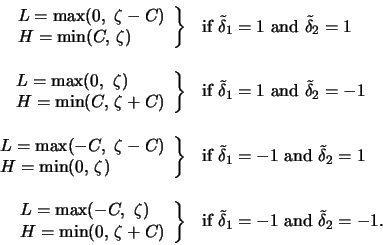
\begin{displaymath}\begin{array}{rl}
\left. \begin{array}{l} L = \max(0,\ \zeta-...
...lta}_1 = -1 \ \textrm{and} \ \tilde{\delta}_2 = -1.
\end{array}\end{displaymath}

Thus, taking

\begin{displaymath}z_1^{o,\, c} = \left\{ \begin{array}{ll}
H & \textrm{if} \ z_...
...1^o \leq H \\
L & \textrm{if} \ z_1^o < L \end{array} \right.
\end{displaymath}

and

\begin{displaymath}z_2^o = \zeta - z_1^{o,\, c}\end{displaymath}

the minimum of (21) under the constraints (22) and (23) is obtained at $(z_1^{o,\, c},\, z_2^o)$ if $\eta > 0$. In the pathological case where $\eta \leq 0$, it is clear that the solution

\begin{displaymath}z_1^o = \left\{ \begin{array}{ll} L & \textrm{if} \ \Lambda(L...
... \textrm{if} \ \Lambda(L) \geq \Lambda(H)
\end{array} \right.
\end{displaymath}

and

\begin{displaymath}z_2^o = \zeta - z_1^o\end{displaymath}

is the minimum.


next up previous
Next: Shrinking Up: The Decomposition Algorithm Previous: Selection of a New
Journal of Machine Learning Research