In this section, we will see that although (single) round robin classification turns a single c-class learning problem into c(c-1)/2 two-class problems, the total training effort is only linear in the number of classes and smaller than the effort needed for an unordered binarization. The analysis is independent of the type of base learning algorithm used, although we will show that the advantage increases with the computational complexity of the algorithm. Some of the ideas have already been sketched in a short paragraph by Friedman (1996), but we go into considerably more detail and, in particular, focus on the comparison to conventional class binarization techniques.
In the following, we assume a base learner with a time complexity
function f(n), i.e., the time needed for learning a classifier from
a training set with n examples is f(n). Note that we
interpret this as an exact function, and not as an
asymptotically tight bound as in
![]() because we are not
interested in asymptotic behavior, but in the exact complexity at a
given training set size n.8 We will consider
functions of the form
because we are not
interested in asymptotic behavior, but in the exact complexity at a
given training set size n.8 We will consider
functions of the form
![]() and denote such a function with
and denote such a function with ![]() . We use b|f to denote a class
binarization with algorithm b, where an base learner with complexity
f(n) is applied to each binary problem. Unless mentioned otherwise,
all results refer to single round robin binarizations of problems with
more than two classes (c > 2).
. We use b|f to denote a class
binarization with algorithm b, where an base learner with complexity
f(n) is applied to each binary problem. Unless mentioned otherwise,
all results refer to single round robin binarizations of problems with
more than two classes (c > 2).
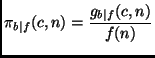
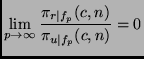
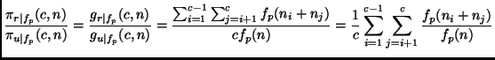
Intuitively, the class penalty
![]() measures the
performance of an algorithm on a class binarized c-class problem
relative to its performance on a single two-class problem the same
size n. In the following, it will turn out that in some cases the
class penalty function is independent of n or f. In such
cases, we will abbreviate the notation as
measures the
performance of an algorithm on a class binarized c-class problem
relative to its performance on a single two-class problem the same
size n. In the following, it will turn out that in some cases the
class penalty function is independent of n or f. In such
cases, we will abbreviate the notation as ![]() .
.
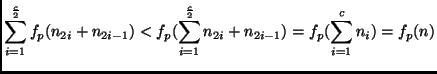
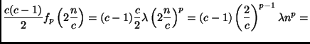
As f is linear, the sum of the complexities on all individual
training sets is equal to the complexity of the algorithm on the sum
of all training set sizes, i.e.,
![]() . Hence,
. Hence,
This analysis ignores a possible constant overhead of the
algorithm, which potentially affects c(c-1)/2 function calls in
the round robin case, while it only affects c function calls in the
unordered case. However, some significant overhead costs, like reading
in the training examples (and similar initialization steps) need, of
course, only be performed once if the round robin procedure is
performed in memory (which was not the case in the implementation
which we used for the experimental results reported in the next
section). If there is an overhead ![]() to be considered (i.e.,
to be considered (i.e.,
![]() ), the total costs will be increased by
), the total costs will be increased by
![]() . For very large values of c, these
quadratic costs may outweigh the savings, but under reasonable
assumptions (e.g.,
. For very large values of c, these
quadratic costs may outweigh the savings, but under reasonable
assumptions (e.g., ![]() ) these additive costs should not matter,
in particular--as we shall see in the following--not in the case of
super-linear base algorithms.
) these additive costs should not matter,
in particular--as we shall see in the following--not in the case of
super-linear base algorithms.
c is even:
In this case, we can arrange the learning tasks in the form of c-1
rounds. Each round consists of c/2 disjoint pairings, i.e.,
each class occurs exactly once in each round, and it has a different
partner in each round. Such a tournament schedule is always
possible.9 Without loss of generality, consider a round where classes
2i are paired against classes 2i-1. The complexity of this round
is
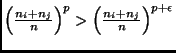
![]() . As for p > 1 and
. As for p > 1 and
![]() , i = 1...N it holds that
, i = 1...N it holds that
![]() , and
because we assumed c > 2, we get
, and
because we assumed c > 2, we get
c is odd:
we add a dummy class with
![]() examples, and perform a tournament as above. As this tournament has
c rounds,
examples, and perform a tournament as above. As this tournament has
c rounds,
![]() .
.
![]()
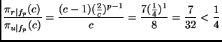
As mentioned above, the bounds used for proving the lemmas are certainly not tight. This becomes obvious, if we look at problems with a uniform class distribution.
 |
|||
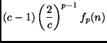 |
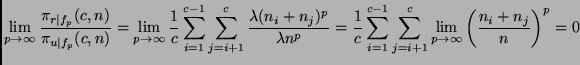
From this result, it is easy to see that
![]() decreases
with increasing complexity order p of the base learner (assuming c
> 2). Likewise, for p > 2,
decreases
with increasing complexity order p of the base learner (assuming c
> 2). Likewise, for p > 2,
![]() can be made arbitrarily small
by increasing the number of classes c. While the latter property is
hard to generalize for arbitrary class distributions--it is not the
case that every problem with more than c classes has a smaller class
penalty than an arbitrary c-class problem (and vice versa)--it is
easy to prove the following theorem:
can be made arbitrarily small
by increasing the number of classes c. While the latter property is
hard to generalize for arbitrary class distributions--it is not the
case that every problem with more than c classes has a smaller class
penalty than an arbitrary c-class problem (and vice versa)--it is
easy to prove the following theorem:
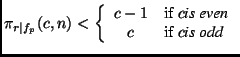
 for all
As the decrease with increasing order p is strictly monotonic, this theorem implies that the more expensive a learning algorithm is, the larger will be the efficiency gain for using round robin binarization instead of unordered binarization. In particular, it may be the case that for expensive algorithms, even a double round robin is faster than unordered binarization (in fact, it is easy to see that Theorem 5.7 also holds for double round robin binarization) or may be even faster than ordered binarization. Assume, e.g., an algorithm with a quadratic complexity on a class-balanced eight-class problem (i.e., p=2 and c = 8). According to Theorem 5.6 and Lemma 5.2: