


Next: Marginalization, inference and sampling
Up: Learning with Mixtures of
Previous: Related work
Tree distributions
In this section we introduce the tree model and the notation that
will be used throughout the paper. Let  denote a set of
 discrete random variables of interest. For each random variable
 let
let  represent its range,
 a
particular value, and
a
particular value, and  the (finite) cardinality of .
For each subset
the (finite) cardinality of .
For each subset  of , let
 and let
  denote an assignment to the variables in .
To simplify notation
denote an assignment to the variables in .
To simplify notation  will be denoted by
  and
and  will be denoted simply by
  . Sometimes we need to refer to the
maximum of over ; we denote this value by
. Sometimes we need to refer to the
maximum of over ; we denote this value by  .
We begin with undirected (Markov random field) representations of tree
distributions. Identifying the vertex set of a graph with the set of
random variables , consider a graph
.
We begin with undirected (Markov random field) representations of tree
distributions. Identifying the vertex set of a graph with the set of
random variables , consider a graph  , where
  is a
set of undirected edges. We allow a tree to have multiple
connected components (thus our ``trees'' are generally called
forests). Given this definition, the number of edges
is a
set of undirected edges. We allow a tree to have multiple
connected components (thus our ``trees'' are generally called
forests). Given this definition, the number of edges  and
the number of connected components
and
the number of connected components  are related as follows:
implying that adding an edge to a tree reduces the number of
connected components by 1. Thus, a tree can have at most  edges. In this latter case we refer to the tree as a spanning
tree.
We parameterize a tree in the following way. For
edges. In this latter case we refer to the tree as a spanning
tree.
We parameterize a tree in the following way. For  and
and
 , let
, let  denote a joint probability distribution on
 and
and  . We require these distributions to be consistent with
respect to marginalization, denoting by
. We require these distributions to be consistent with
respect to marginalization, denoting by  the marginal of
 or
or
 with respect to
  for any
 . We now assign a distribution
  to the graph
 as follows:
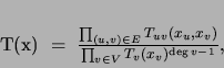 |
(1) |
where deg is the degree of vertex ; i.e., the number of
edges incident to . It can be verified that is in
fact a probability distribution; moreover, the pairwise probabilities
are the marginals of .
A tree distribution is defined to be any distribution
that admits a factorization of the form (1).
Tree distributions can also be represented using directed (Bayesian
network) graphical models. Let
is the degree of vertex ; i.e., the number of
edges incident to . It can be verified that is in
fact a probability distribution; moreover, the pairwise probabilities
are the marginals of .
A tree distribution is defined to be any distribution
that admits a factorization of the form (1).
Tree distributions can also be represented using directed (Bayesian
network) graphical models. Let  denote a directed
tree (possibly a forest), where
denote a directed
tree (possibly a forest), where  is a set of directed edges and
where each node has (at most) one parent, denoted pa
is a set of directed edges and
where each node has (at most) one parent, denoted pa .
We parameterize this graph as follows:
.
We parameterize this graph as follows:
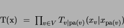 |
(2) |
where
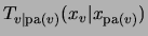 is an arbitrary
conditional distribution. It can be verified that indeed
defines a probability distribution; moreover, the marginal
conditionals of are given by the conditionals
is an arbitrary
conditional distribution. It can be verified that indeed
defines a probability distribution; moreover, the marginal
conditionals of are given by the conditionals
 .
We shall call the representations (1) and
(2) the undirected and directed tree
representations of the distribution respectively. We can
readily convert between these representations; for example, to
convert (1) to a directed representation we choose
an arbitrary root in each connected component and direct each
edge away from the root. For with closer to
the root than , let pa
.
We shall call the representations (1) and
(2) the undirected and directed tree
representations of the distribution respectively. We can
readily convert between these representations; for example, to
convert (1) to a directed representation we choose
an arbitrary root in each connected component and direct each
edge away from the root. For with closer to
the root than , let pa . Now compute the conditional
probabilities corresponding to each directed edge by recursively
substituting
. Now compute the conditional
probabilities corresponding to each directed edge by recursively
substituting
 by
by
 starting from the root.
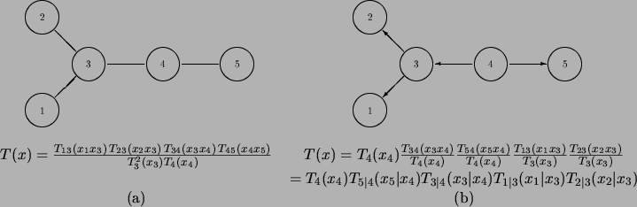
Figure 2 illustrates this process on a tree with
5 vertices.
starting from the root.
Figure 2 illustrates this process on a tree with
5 vertices.
Figure 2:
A tree in its undirected (a) and directed (b) representations.
 |
The directed tree representation has the advantage of having
independent parameters. The total number of free parameters in either
representation is:
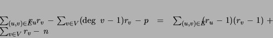 |
(3) |
The right-hand side of (3) shows that each edge
 increases the number of parameters by
 .
The set of conditional independencies associated with a tree
distribution are readily characterized [Lauritzen, Dawid, Larsen, Leimer
1990].
In particular, two subsets
.
The set of conditional independencies associated with a tree
distribution are readily characterized [Lauritzen, Dawid, Larsen, Leimer
1990].
In particular, two subsets  are independent given
 if
if  intersects every path (ignoring the direction
of edges in the directed case) between and for all
intersects every path (ignoring the direction
of edges in the directed case) between and for all  and
and  .
.
Subsections
Next: Marginalization, inference and sampling
Up: Learning with Mixtures of
Previous: Related work
Journal of Machine Learning Research
2000-10-19