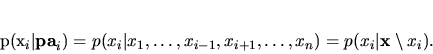
Theorem 1: The set of positive distributions that can
be encoded by a consistent dependency network with graph ![]() is
equal to the set of positive distributions that can be encoded by a
Markov network whose structure has the same adjacencies as
is
equal to the set of positive distributions that can be encoded by a
Markov network whose structure has the same adjacencies as ![]() .
.
The two graphical representations are different in that
Markov networks quantify dependencies with potential functions,
whereas dependency networks use conditional probabilities. We have
found the latter to be significantly easier to interpret.
The proof of Theorem 1 appears in the Appendix, but it is essentially
a restatement of the Hammersley-Clifford theorem (e.g., Besag, 1974).
This correspondence is no coincidence. As is discussed in Besag
(1974), several researchers who developed the Markov-network
representation did so by initially investigating a graphical
representation that fits our definition of consistent dependency
network. In particular, several researchers including Lévy
(1948), Bartlett (1955, Section
2.2), and Brook (1964) considered
lattice systems where each variable ![]() depended only on its nearest
neighbors
depended only on its nearest
neighbors ![]() , and quantified the dependencies within these systems
using the conditional probability distributions
, and quantified the dependencies within these systems
using the conditional probability distributions
![]() . They
then showed, to various levels of generality, that the only joint
distributions mutually consistent with each of the conditional
distributions also satisfy Equation 2. Hammersley
and Clifford, in a never published manuscript, and Besag
(1974) considered the more general case where each
variable could have an arbitrary set of parents. They showed that,
provided the joint distribution for
. They
then showed, to various levels of generality, that the only joint
distributions mutually consistent with each of the conditional
distributions also satisfy Equation 2. Hammersley
and Clifford, in a never published manuscript, and Besag
(1974) considered the more general case where each
variable could have an arbitrary set of parents. They showed that,
provided the joint distribution for ![]() is positive, any graphical
model specifying the independencies in Equation 1 must also
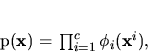
satisfy Equation 2. One interesting point is that
these researchers argued for the use of conditional distributions to
quantify the dependencies. They considered the resulting potential
form in Equation 2 to be a mathematical necessity
rather than a natural expression of dependency. As we have just
discussed, we share this view.
The equivalence of consistent dependency networks and Markov networks
suggests a straightforward approach for learning a consistent
dependency network from exchangeable (i.i.d.) data. Namely, one
learns the structure and potentials of a Markov network (e.g.,
Whittaker, 1990), and then computes (via
probabilistic inference) the conditional distributions required by the
dependency network. Alternatively, one can learn a related model such
as a Bayesian network, decomposable model, or hierarchical log-linear
model (see, e.g., Lauritzen, 1996) and convert it
to a consistent dependency network. Unfortunately, the conversion
process can be computationally expensive in many situations. In the
next section, we extend the definition of dependency network to
include inconsistent dependency networks and provide algorithms for
learning such networks that are more computationally efficient than
those just described. In the remainder of this section, we apply well
known results about probabilistic inference to consistent dependency
networks. This discussion will be useful for our further development
of (general) dependency networks.
is positive, any graphical
model specifying the independencies in Equation 1 must also
satisfy Equation 2. One interesting point is that
these researchers argued for the use of conditional distributions to
quantify the dependencies. They considered the resulting potential
form in Equation 2 to be a mathematical necessity
rather than a natural expression of dependency. As we have just
discussed, we share this view.
The equivalence of consistent dependency networks and Markov networks
suggests a straightforward approach for learning a consistent
dependency network from exchangeable (i.i.d.) data. Namely, one
learns the structure and potentials of a Markov network (e.g.,
Whittaker, 1990), and then computes (via
probabilistic inference) the conditional distributions required by the
dependency network. Alternatively, one can learn a related model such
as a Bayesian network, decomposable model, or hierarchical log-linear
model (see, e.g., Lauritzen, 1996) and convert it
to a consistent dependency network. Unfortunately, the conversion
process can be computationally expensive in many situations. In the
next section, we extend the definition of dependency network to
include inconsistent dependency networks and provide algorithms for
learning such networks that are more computationally efficient than
those just described. In the remainder of this section, we apply well
known results about probabilistic inference to consistent dependency
networks. This discussion will be useful for our further development
of (general) dependency networks.