The SPLICE dataset: Classification

We also studied the classification performance of the MT model in the domain of DNA SPLICE-junctions. The domain consists of 60 variables, representing a sequence of DNA bases, and an additional class variable [Rasmussen 1996]. The task is to determine if the middle of the sequence is a splice junction and what is its type. Splice junctions are of two types: exon-intron (EI) represents the end of an exon and the beginning of an intron whereas intron-exon (IE) is the place where the intron ends and the next exon, or coding section, begins. Hence, the class variable can take 3 values (EI, IE or no junction) and the other variables take 4 values corresponding to the 4 possible DNA bases (C, A, G, T). The dataset consists of 3,175 labeled examples.² We ran two series of experiments comparing the MT model with competing models. In the first series of experiments, we compared to the results of noordewier:91, who used multilayer neural networks and knowledge-based neural networks for the same task. We replicated these authors' choice of training set size (2000) and test set size (1175) and sampled new training/test sets for each trial. We constructed trees ($m=1$) and mixtures of trees ($m=3$). In fitting the mixture, we used an early-stopping procedure in which $N_{valid}$=300 examples were separated out of the training set and training was stopped when the likelihood on these examples stopped increasing. The results, averaged over 20 trials, are presented in Figure 15 for a variety of values of $\alpha$. It can be seen that the single tree and the MT model perform similarly, with the single tree showing an insignificantly better classification accuracy. Note that in this situation smoothing does not improve performance; this is not unexpected since the data set is relatively large. With the exception of the ``oversmoothed'' MT model ($\alpha=100$), all the single tree or MT models outperform the other models tested on this problem. Note that whereas the tree models contain no prior knowledge about the domain, the other two models do: the neural network model is trained in supervised mode, optimizing for class accuracy, and the KBNN includes detailed domain knowledge. Based on the strong showing of the single tree model on the SPLICE task, we pursued a second series of experiments in which we compare the tree model with a larger collection of methods from the DELVE repository [Rasmussen, 1996]. The DELVE benchmark uses subsets of the SPLICE database with 100 and 200 examples for training. Testing is done on 1500 examples in all cases. Figure 16 presents the results for the algorithms tested by DELVE as well as the single trees with different degrees of smoothing. We also show results for naive Bayes (NB) and Tree Augmented Naive Bayes (TANB) models [Friedman, Geiger, Goldszmidt 1997]. The results from DELVE represent averages over 20 runs with different random initializations on the same training and testing sets; for trees, NB and TANB, whose outputs are not initialization-dependent, we averaged the performance of the models learned for 20 different splits of the union of the training and testing set. No early stopping or cross-validation was used in this case.

Figure 17: Cumulative adjacency matrix of 20 trees fit to 2000 examples of the SPLICE data set with no smoothing. The size of the square at coordinates $ij$ represents the number of trees (out of 20) that have an edge between variables $i$ and $j$. No square means that this number is 0. Only the lower half of the matrix is shown. The class is variable 0. The group of squares at the bottom of the figure shows the variables that are connected directly to the class. Only these variable are relevant for classification. Not surprisingly, they are all located in the vicinity of the splice junction (which is between 30 and 31). The subdiagonal ``chain'' shows that the rest of the variables are connected to their immediate neighbors. Its lower-left end is edge 2-1 and its upper-right is edge 60-59.

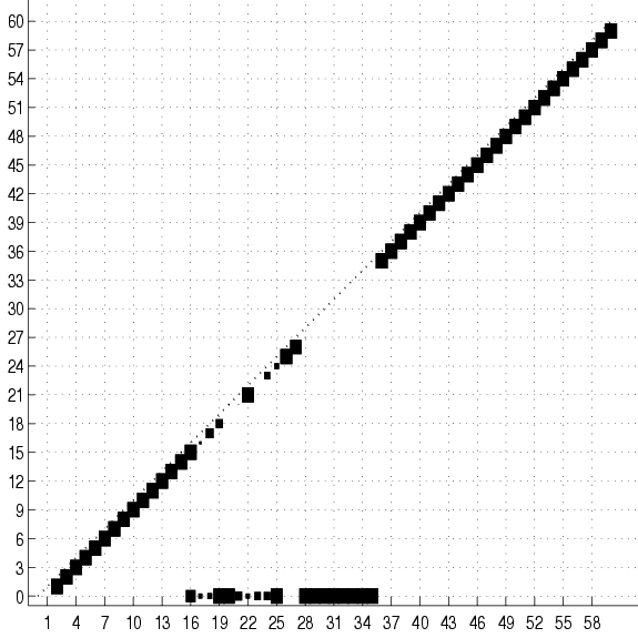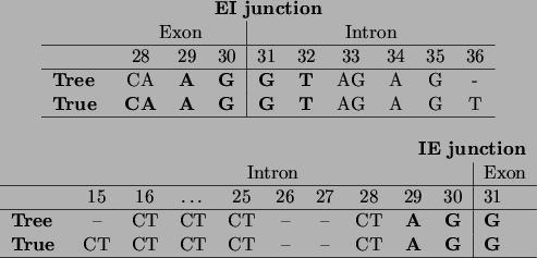
Figure 18: The encoding of the IE and EI splice junctions as discovered by the tree learning algorithm, compared to the ones given by Watson et al., ``Molecular Biology of the Gene'' [Watson, Hopkins, Roberts, Steitz, Weiner 1987]. Positions in the sequence are consistent with our variable numbering: thus the splice junction is situated between positions 30 and 31. Symbols in boldface indicate bases that are present with probability almost 1, other A,C,G,T symbols indicate bases or groups of bases that have high probability ($>$0.8), and a - indicates that the position can be occupied by any base with a non-negligible probability.

The results show that the single tree is quite successful in this domain, yielding an error rate that is less than half of the error rate of the best model tested in DELVE. Moreover, the average error of a single tree trained on 200 examples is 6.9%, which is only 2.3% greater than the average error of the tree trained on 2000 examples. We attempt to explain this striking preservation of accuracy for small training sets in our discussion of feature selection in Section 5.3.7. The Naive Bayes model exhibits behavior that is very similar to the tree model and only slightly less accurate. However, augmenting the Naive Bayes model to a TANB significantly hurts the classification performance.

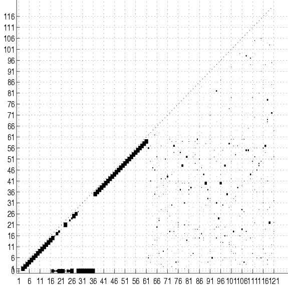
Figure 19: The cumulated adjacency matrix for 20 trees over the original set of variables (0-60) augmented with 60 ``noisy'' variables (61-120) that are independent of the original ones. The matrix shows that the tree structure over the original variables is preserved.