


Next: Near Consistency: Theoretical Considerations
Up: General Dependency Networks
Previous: Probabilistic Decision Trees for
Probabilistic Inference With Real Data
We have suggested that, because the local distributions learned from
data sets of adequate size will be close to the true underlying
distribution and hence almost consistent, the procedures for
extracting a joint distribution from a dependency network and for
answering probabilistic queries should yield fairly accurate results.
Nonetheless, there is a concern. It could be that the application of
pseudo-Gibbs sampling amplifies the inconsistencies. That is, it
could be that small perturbations from the true conditional
distributions
 could lead to large
perturbations from the true joint distribution
could lead to large
perturbations from the true joint distribution  . If this
phenomenon did occur, it is likely that predictions of new data
rendered by a dependency network would be inaccurate. In this
section, we compare the predictions of dependency networks and
Bayesian networks on real data sets as a first examination of this
concern.
We use four datasets: (1) Sewall/Shah, data from Sewall and Shah
(1968) regarding the college plans of high-school
seniors, (2) Women and Mathematics (WAM), data regarding women's
preferences for a career in Mathematics (Fowlkes, Freeny, and
Landwehr, 1988), (3) Digits, images of handwritten
digits made available by the US Postal Service Office for Advanced
Technology (Frey, Hinton, and Dayan, 1995), and (4)
Nielsen, data about whether or not users watched five or more minutes
of network TV shows aired during a two-week period in 1995 (made
available by Nielsen Media Research). In each of these datasets, all
variables are finite. For the digits data, we report results for only
two (randomly chosen) digits, ``2'' and ``6''. Additional details
about the datasets are given in Table 1.
To evaluate the accuracy of dependency networks on these datasets, we
randomly partition each dataset into a training set and a test set
used to learn models and evaluate them, respectively. We measure the
accuracy of each learned model on the test set
. If this
phenomenon did occur, it is likely that predictions of new data
rendered by a dependency network would be inaccurate. In this
section, we compare the predictions of dependency networks and
Bayesian networks on real data sets as a first examination of this
concern.
We use four datasets: (1) Sewall/Shah, data from Sewall and Shah
(1968) regarding the college plans of high-school
seniors, (2) Women and Mathematics (WAM), data regarding women's
preferences for a career in Mathematics (Fowlkes, Freeny, and
Landwehr, 1988), (3) Digits, images of handwritten
digits made available by the US Postal Service Office for Advanced
Technology (Frey, Hinton, and Dayan, 1995), and (4)
Nielsen, data about whether or not users watched five or more minutes
of network TV shows aired during a two-week period in 1995 (made
available by Nielsen Media Research). In each of these datasets, all
variables are finite. For the digits data, we report results for only
two (randomly chosen) digits, ``2'' and ``6''. Additional details
about the datasets are given in Table 1.
To evaluate the accuracy of dependency networks on these datasets, we
randomly partition each dataset into a training set and a test set
used to learn models and evaluate them, respectively. We measure the
accuracy of each learned model on the test set
 using the log score:
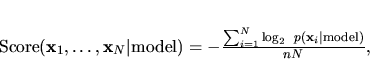 |
(3) |
where  is the number of variables in
  . This score can be
thought of as the average number of bits needed to encode the
observation of a variable in the test set. Note that we measure how
well a dependency network predicts an entire case. We could look at
predictions of particular conditional probabilities, but because
Algorithm 1 uses products of queries to produce a prediction on a full
case, we expect comparisons on individual queries to be similar.
In our experiments, we determine the probabilities
. This score can be
thought of as the average number of bits needed to encode the
observation of a variable in the test set. Note that we measure how
well a dependency network predicts an entire case. We could look at
predictions of particular conditional probabilities, but because
Algorithm 1 uses products of queries to produce a prediction on a full
case, we expect comparisons on individual queries to be similar.
In our experiments, we determine the probabilities
 in Equation 3 from a learned dependency network
using Algorithm 1. For each pseudo-Gibbs sampler invoked in
Algorithm 1, we average 5000 iterations after a 10-iteration burn-in.
For each data set, these Gibbs-sampling parameters yield scores with a
range of variation of less than 0.1% across 10 runs starting with
different (random) initial states.
For comparison, we measure the accuracy of two additional model
classes: (1) a Bayesian network, and (2) a Bayesian network with no
arcs--a baseline model. When learning the non-baseline
Bayesian network, we use the algorithm described in Chickering,
Heckerman, and Meek (1997) wherein each local distribution consists of
a decision tree with binary splits. We use the same parameter and
structure priors as used in the learning of dependency networks. We
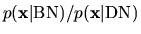
determine
from a Bayesian network using the law
of total probability--pseudo-Gibbs sampling is not needed.
Probability estimates obtained from both Bayesian networks and
dependency networks correspond to the a posteriori mean of the
(multinomial) parameters.
The results are shown in Table 1. The Bayesian networks produce
density estimates that are better than those of dependency networks,
but only slightly so. In particular, consider the summary score in
the second row from the bottom of the table,
in Equation 3 from a learned dependency network
using Algorithm 1. For each pseudo-Gibbs sampler invoked in
Algorithm 1, we average 5000 iterations after a 10-iteration burn-in.
For each data set, these Gibbs-sampling parameters yield scores with a
range of variation of less than 0.1% across 10 runs starting with
different (random) initial states.
For comparison, we measure the accuracy of two additional model
classes: (1) a Bayesian network, and (2) a Bayesian network with no
arcs--a baseline model. When learning the non-baseline
Bayesian network, we use the algorithm described in Chickering,
Heckerman, and Meek (1997) wherein each local distribution consists of
a decision tree with binary splits. We use the same parameter and
structure priors as used in the learning of dependency networks. We
determine
from a Bayesian network using the law
of total probability--pseudo-Gibbs sampling is not needed.
Probability estimates obtained from both Bayesian networks and
dependency networks correspond to the a posteriori mean of the
(multinomial) parameters.
The results are shown in Table 1. The Bayesian networks produce
density estimates that are better than those of dependency networks,
but only slightly so. In particular, consider the summary score in
the second row from the bottom of the table,
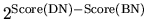 , which is the geometric mean of
 averaged over all cases in a dataset. For
Digit2, the data set having the worst dependency-network performance,
the dependency network assigns a probability to a case, on (geometric)
average, that is only 3% lower than that assigned by the Bayesian
network.
averaged over all cases in a dataset. For
Digit2, the data set having the worst dependency-network performance,
the dependency network assigns a probability to a case, on (geometric)
average, that is only 3% lower than that assigned by the Bayesian
network.
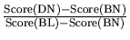
Table 1:
Details for datasets and Score (bits per observation) for a
Bayesian network (BN), dependency network (DN), and baseline model
(BL) applied to these datasets. The lower the Score, the higher the
accuracy of the learned model.
| |
Dataset |
| |
Sewall/Shah |
WAM |
Digit2 |
Digit6 |
Nielsen |
| Number of variables |
5 |
6 |
64 |
64 |
203 |
| Training cases |
9286 |
790 |
700 |
700 |
1637 |
| Test cases |
1032 |
400 |
399 |
400 |
1637 |
| Score(BN) |
1.274 |
0.907 |
0.542 |
0.422 |
0.188 |
| Score(DN) |
1.277 |
0.911 |
0.584 |
0.454 |
0.189 |
| Score(BL) |
1.382 |
0.930 |
0.823 |
0.752 |
0.231 |
| Score(DN)-Score(BN) |
0.002 |
0.004 |
0.042 |
0.033 |
0.001 |
| Score(BL)-Score(BN) |
0.107 |
0.022 |
0.281 |
0.330 |
0.044 |
|
|
1.00 |
1.00 |
1.03 |
1.02 |
1.00 |
 |
0.02 |
0.16 |
0.15 |
0.10 |
0.02 |
That dependency networks are (slightly) less accurate than Bayesian
networks is not surprising. In each domain, the number of parameters
in the Bayesian network are fewer than the number of parameters in the
corresponding dependency network. Consequently, the
dependency-network estimates should have higher variance. This
explanation is consistent with the observation that, roughly,
differences in accuracy are larger for the data sets with smaller
sample size.
Because dependency networks produce joint probabilities via
pseudo-Gibbs sampling whereas Bayesian networks produce joint
probabilities via multiplication, non-convergence of sampling is
another possible explanation for the greater accuracy of Bayesian
networks. The small variances of the pseudo-Gibbs-sampler estimates
across multiple runs, however, makes this explanation unlikely.
Overall, our experiments suggest that Algorithm 1 applied to
inconsistent dependency networks learned from data yields accurate
joint probabilities.
Finally, let us consider issues of computation. Joint estimates
produced by dependency networks require far more computation than do
those produced by Bayesian networks. For example, on a 600 MHz
Pentium III with 128 MB of memory running the Windows 2000 operating
system, the determination of for a case in the Nielsen
dataset takes on average 2.0 seconds for the dependency network and
0.0006 seconds for the Bayesian network. Consequently, one should use
a Bayesian network in those situations where it is known in advance
that joint probabilities are needed. Nonetheless, in
situations where general probabilistic inference is needed, exact
inference in a Bayesian network is often intractable; and
practitioners often turn to Gibbs sampling for inference. In such
situations, Bayesian networks afford little computational advantage.
Next: Near Consistency: Theoretical Considerations
Up: General Dependency Networks
Previous: Probabilistic Decision Trees for
Journal of Machine Learning Research,
2000-10-19