Appendix: Proofs of Theorems

Theorem 1: The set of positive distributions that can be encoded by consistent dependency networks with graph ${\cal G}$ is equal to the set of positive distributions that can be encoded by Markov networks whose structure have the same adjacencies as those in ${\cal G}$.

Proof: Let $p$ be a positive distribution defined by a Markov network where ${\bf A}_i$ are the adjacencies of $X_i$, $i=1,\ldots,n$. Construct a consistent dependency network from $p$ by extracting the conditional distributions $p(x_i\vert{\bf x}\setminus x_i), i=1,\ldots,n$. Because these probabilities came from the Markov network, we know that $p(x_i\vert{\bf x}\setminus x_i) = p(x_i \vert {\bf A}_i), i=1,\ldots,n$ so that the adjacencies in the dependency-network structure are the same as those in the Markov network. Now let $p$ be a positive distribution encoded by a consistent dependency network. By definition, we have that $X_i$ is independent of ${\bf X}\setminus X_i$ given ${\bf Pa}_i$, $i=1,\ldots,n$. Because $p$ is positive and these independencies comprise the global Markov property of a Markov network with ${\bf A}_i={\bf Pa}_i$, $i=1,\ldots,n$, the Hammersley-Clifford theorem (Besag, 1974; Lauritzen, Dawid, Larsen, and Leimer, 1990) implies that $p$ can be represented by this Markov network. $\Box$

Theorem 2: An ordered Gibbs sampler applied to a consistent dependency network for ${\bf X}$, where each $X_i$ is finite (and hence discrete) and each local distribution $p(x_i\vert{\bf pa}_i)$ is positive, defines a Markov chain with a unique stationary joint distribution for ${\bf X}$ equal to $p({\bf X})$ that can be reached from any initial state of the chain.

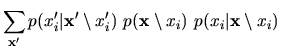
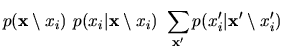
Proof: In the body of the paper, we showed that the Markov chain can be described by the transition matrix ${\bf P}= {\bf P}^1 \cdot \ldots \cdot {\bf P}^n$, where ${\bf P}^k$ is the ``local'' transition matrix describing the resampling of $X_k$ according to the local distribution $p(x_k\vert{\bf pa}_k)$. We also showed that this Markov chain has a unique joint distribution that can be reached from any starting point. Here, we show that $p({\bf x})$ is that stationary distribution--that is, $p({\bf x}) = \sum_{{\bf x}'} p({\bf x}') \ {\bf P}_{{\bf x}\vert{\bf x}'}$, where ${\bf P}_{{\bf x}\vert{\bf x}'} = p({\bf x}^{t+1}={\bf x}'\vert{\bf x}^{t}={\bf x})$. To do so, we show that for each ${\bf P}^i$, $p({\bf x}) = \sum_{{\bf x}'} p({\bf x}') \ {\bf P}^i_{{\bf x}\vert{\bf x}'}$.

$${\sum_{{\bf x}'} p({\bf x}') \ {\bf P}^i_{{\bf x}\vert{\bf x}'}} = {\sum_{{\bf x}'} p(x_i' \vert {\bf x}' \setminus x_i') \ p({\bf x}' \setminus x_i') \ {\bf P}^i_{{\bf x}\vert{\bf x}'}}$$ (11)

$$= {\sum_{{\bf x}'} p(x_i' \vert {\bf x}' \setminus x_i') \ p({\bf x}' \setminus x_i') \ p(x_i \vert {\bf pa}_i')}$$ (12)

$$= {\sum_{{\bf x}'} p(x_i' \vert {\bf x}' \setminus x_i') \ p({\bf x}' \setminus x_i') \ p(x_i \vert {\bf x}' \setminus x_i')}$$ (13)

$$= {\sum_{{\bf x}'} p(x_i' \vert {\bf x}' \setminus x_i') \ p({\bf x}\setminus x_i) \ p(x_i \vert {\bf x}\setminus x_i)}$$ (14)

$$= p({\bf x}\setminus x_i) \ p(x_i \vert {\bf x}\setminus x_i) \ \sum_{{\bf x}'} p(x_i' \vert {\bf x}' \setminus x_i')$$ (15)

$$= p({\bf x})$$ (16)

Equation 12 follows from Equation 11 using the definition of ${\bf P}^i$. Equation 13 follows from Equation 12 using the definition of a consistent dependency network. Equation 14 follows from Equation 13 by observing that the value of ${\bf x}$ and ${\bf x}'$ can differ only in variable $x_i$. The other steps are straightforward.$\Box$

Theorem 4: A minimal consistent dependency network for a positive distribution $p({\bf x})$ must be bi-directional.

Proof: We use the graphoid axioms of Pearl (1988). Suppose the theorem is false. Then, there exists nodes $X_i$ and $X_j$ such that $X_j$ is a parent of $X_i$ and $X_i$ is not a parent of $X_j$. Let ${\bf Z}= {\bf Pa}_i\cap {\bf Pa}_j$, ${\bf W}={\bf Pa}_i \setminus ({\bf Pa}_j\cup \{X_j\})$, and ${\bf Y}= {\bf Pa}_j\setminus {\bf Pa}_i$. From minimality, we know that $X_i\mbox{$\perp\! \perp$}X_j\mbox{$\vert$}{\bf W},{\bf Z}$ does not hold. By decomposition, $X_i\mbox{$\perp\! \perp$}X_j,{\bf Y}\mbox{$\vert$}{\bf W},{\bf Z}$ does not hold. Given positivity, the intersection property holds. By the intersection property, at least one of the following conditions does not hold: (1) $X_i\mbox{$\perp\! \perp$}X_j\mbox{$\vert$}{\bf W},{\bf Y},{\bf Z}$, (2) $X_i\mbox{$\perp\! \perp$}{\bf Y}\mbox{$\vert$}X_j,{\bf W},{\bf Z}$. (If ${\bf Y}= \emptyset$, then condition 2 holds vacuously.) Now, from Theorem 2, we know that $X_i,{\bf W}\mbox{$\perp\! \perp$}X_j\mbox{$\vert$}{\bf Y},{\bf Z}$. Using weak union, we have that $X_i\mbox{$\perp\! \perp$}X_j\mbox{$\vert$}{\bf W},{\bf Y},{\bf Z}$--that is, condition 1 holds. Also, from Theorem 2, we know that $X_i\mbox{$\perp\! \perp$}{\bf Y}\mbox{$\vert$}X_j,{\bf W},{\bf Z}$--that is, condition 2 holds, yielding a contradiction. $\Box$